Environment design in Blender
Recently, I got into creating 3D environments in Blender. While it involves a lot of artistic elements, there are some rules and workflows that make the process easier. I watched dozens of youtube tutorials about the topic and wrote down the lessons I learned in this post. Warning: this is a long read.
Idea
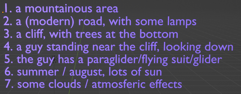
Environment creation starts with an idea. To develop the workflow for building the landscapes, I came up with two environments: a desert and a mountain.
For the desert one, I was initially planning to have an animation with a person hiding and shooting a bow in the direction of another character. For the mountainous area, it was meant to be an animation of a character in a wingsuit starting to fly down a road.
I wrote down the elements in the scene, what mood it would have, etc. It helps in focusing and acts as a reference point for later. Of course, the final landscape may differ from the initial idea based on how it goes.
I looked at some options for storing the idea in the blender file. One of them was a Blender plugin that allows extra “note properties” on an object, but I ended up making a “Text” object and setting it as not-to-render. It wasn’t very convenient, but it was the best thing I tried.
Workflow
Converting an idea to the final environment involves a lot of steps. While making the two landscapes, I divided the process into a couple of stages:
- collecting references
- drawing a map of the terrain
- modelling a mesh of the landscape
- texturing the mesh
- adding repeating elements: trees, grass, rocks
- lighting the scene
- adding a character
- choosing the camera settings
- adding atmospheric effects and clouds
- bringing some assets close to the camera: tree branches, weapons, dice, etc.
Each of them is a separate topic to explore. In the following sections, I detail what I learned about them.
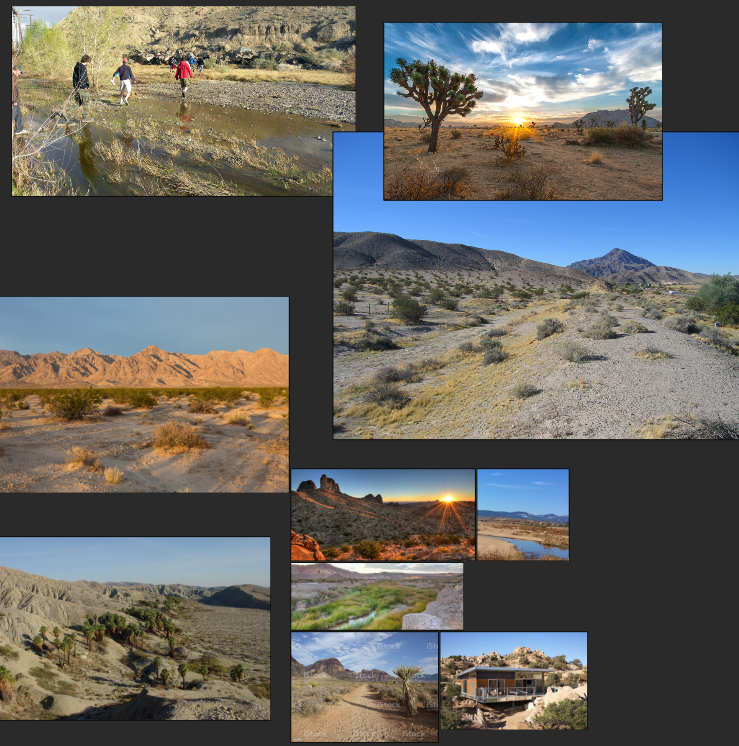
References
When designing a landscape (or anything visual), it’s useful to collect references on how similar objects look in the real world. Humans’ visual memory tends to be vague and forgets the details quickly.
PureRef is a popular tool for storing references. It stores photos that one finds on the internet and allows one to move the board around. It doesn’t have a lot of options, but it serves its purpose well.
Map
I started creating a landscape by drawing a rough sketch of a map of the terrain to mark where there will be a mountain, a river, etc.
To do that, I used Blender’s annotate tool. It didn’t work as well as I’d like to: once drawn, it was difficult to turn the annotations on and off, and I also had some problems making sure that I’m drawing on the right plane, but it was good enough for a rough sketch.
Drawing a map with a mouse would be painful, so instead, I connected my ipad as a graphic screen using weylus and used the apple pencil to create the map in Blender.
Creating mesh of the landscape
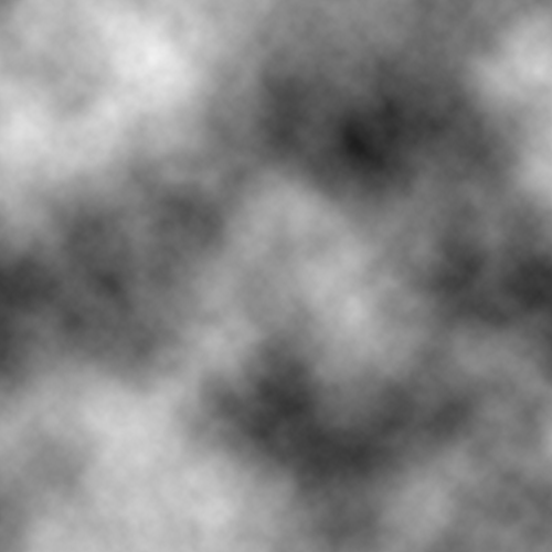
Mesh is the set of vertices and connecting them edges used to describe a shape of a 3D object. For creating landscapes (in particular mountains), creating the mesh manually by simulating clay sculpting would be tedious: a lot of detail is needed for the model to look plausible.
Fortunately, there are mathematical tools that procedurally generate useful landscape meshes out of random noise. The most popular of them is Perlin noise, which puts random values, defining the height of the landscape, smoothly on a 2D surface. The noise consists of a number of noise octaves: the lower-frequency ones define the general shape of the terrain, whereas the higher-frequency ones express smaller bumps.
Generating landscape in Blender
There are two ways to create a landscape using Perlin noise in Blender: directly through noise texture node, and using Another Noise Tool add-on.
Displacement
When using the noise texture node, we are given a plane with the noise and pass it as a displacement in the shader, telling the renderer to modify the mesh using the (generated) texture.
This setting gives the artist a lot of control over how the final mesh looks but requires some knowledge and tinkering to create anything beyond a generic mountain.
For the displacement to actually modify the mesh (as opposed to only altering how the light bounces off of the original surface), one needs to use the Cycles rendering engine and set Displacement only in Material > Settings > Displacement.
Another Noise Tool
The A.N.T. add-on simplifies the process of landscape generation by storing several randomness settings corresponding to various terrains. After choosing a default to base the environment on, one can further alter the settings to change the random seed or increase the height or water level of the landscape.
Generally, the A.N.T. tool is easy to use and allows to create landscapes more quickly than using the texture noise directly. I have encountered two problems when using it, though:
- As one chooses the noise settings from the operator box1, the landscape has to be finished in a single step. Clicking outside of the box will close it, and bringing it back (with F9) is only possible before making any other operations (even if they are unrelated to the landscape).
- Scaling up the landscape requires changing multiple parameters: to be able to change the size of the whole object, one needs to modify the size of the mesh, the size of the “random noise”, as well as alter the height of the terrain. While it makes sense for these settings to be separate (one may want to increase the X-Y size of the mesh without changing the height), a single slider for scaling the landscape up would be more convenient. It is particularly painful given the previous point, as it isn’t possible to scale the landscape up by the standard means and continue modifying the noise parameters.
Whether using the noise texture or the add-on, one needs to be careful with the number of vertices of the created mesh. While more detailed meshes look better, I observed that anything beyond 256x256 slows down the whole workflow significantly.
In the case of the mountainous terrain, to preserve high detail at the peaks (where I also placed snow, which made the lack of details very apparent) I subdivided only parts of the meshes corresponding to the more visible areas near the peaks. This way, I had more vertices where needed without significantly increasing the overall number.
Water
Some form of water (ocean, river, lake) is a frequent guest on a landscape. Blender has a built-in modifier that deforms a plane to simulate water waves. It has many settings; I haven’t played with them a lot2 but was able to get a convincing-looking mesh after a bit of tinkering.
One problem I had with the water was that the water looked nice and reflective while using the material preview but completely dark during rendering.
After watching some tutorials on the matter, I saw that to make water more glossy, people mark it as highly metallic in the Principled BSDF3, even though it doesn’t make physical sense.
Texturing
Once the mesh is finished, one needs to put a texture with colors on top of it. For standard materials, like wood, brick, gravel, or snow, many websites allow downloading textures for free, e.g.
As the texture is two-dimensional, but the mesh vertices are three-dimensional objects, one needs to map each vertex to the corresponding place on the texture in the process of UV unwrapping.
In Blender, there are two mechanisms for modifying this mapping:
- By modifying the UV map itself, changing how parts of the texture are stretched and expanded to fit the mesh. In the case of the landscape, the automatically generated UV map worked just fine, as with the texture containing generic materials it doesn’t matter where different parts of it get applied (as opposed to unwrapping a texture of a human model, where we don’t want the leg texture to appear on the head).
- By making changes to the material’s shader (function mapping vertices to colors), allowing to apply mathematical transformations to the textures, combining multiple textures, etc. I used this part extensively.
Modifying the UV mapping in the shader
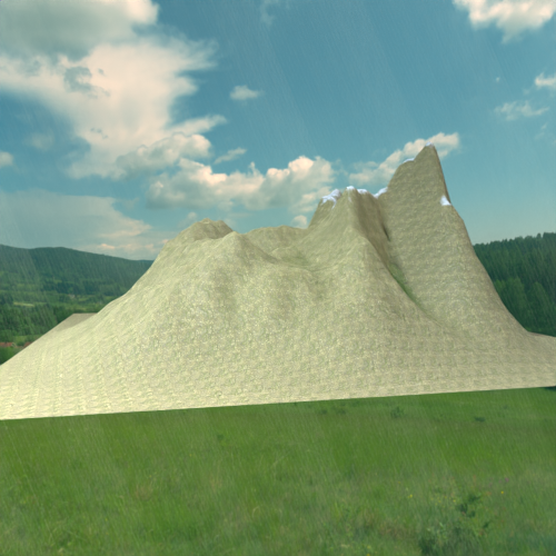
While the textures one can get for free are usually high quality (4 or 8K4), in a sense they are both too small and too big. They are too small, as they aren’t able to cover a large mountain in full: unwrapping the texture once (with no repetitions) over the mesh will cause the smaller elements of the material (like grass, or rocks) to look too big in proportion:
At the same time, the high-density textures are resource-heavy, causing the rendering process to use more memory and become slower.
The common solution to this problem is to use a given texture image multiple times in different places of the mesh: as the texture is of a material, it doesn’t matter where exactly a given part of the texture is being placed, and whether all parts of the material are unique, as long as the repetitions are not blatant.
To achieve that, Blender’s image texture node, which is part of the shader, receives a location input. Using it, one can arbitrarily change the mapping between the vertices in the mesh and the positions on the texture.
To repeat the texture multiple times, one needs to scale the location input by a number bigger than 1: for example, if it is scaled by 2, the 0-1 coordinates in the UV map will correspond to 0-2 on the texture, repeating the texture twice along each axis.
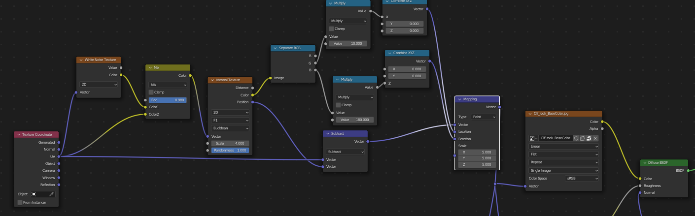
Texture Coordinate node
The shader is a mapping from the mesh vertices to the colors. In our case, the vertices are mapped to a position on the texture5.
By default, the location used for a given vertex is expressed as its two-dimensional coordinates on the UV map: the 3D vertex is mapped to 2D by the UV map, and the further operations: modifying colors or scaling, are applied in two dimensions only.
One may want to use a different coordinate system for representing the vertices in the shader: for example, if one doesn’t have a UV map, and wants to use the actual, 3D coordinates of the vertices in the world, process them, and pass them as the input to the image texture node.
To change the coordinate system of vertices’ in the shader, Blender has a Texture Coordinate node.
Typical shader setup, where the UV coordinates of the vertices are transformed by a vector mapping before being used to choose a place in a texture.
Various outputs of the Texture Coordinate node correspond to different coordinate systems in which vertices can be expressed. The more useful ones are defined as follows:
- UV: the default system, where the vertices are represented as their (2D) coordinates on the UV map.
- Generated: the coordinate system of the smallest bounding box of the object. For each vertex, it will output (three-dimensional, each from 0 to 1) coordinates describing where in the bounding box the vertex lies6.
- Object: the coordinates of the vertices relative to the position of another object.
- Normal: outputs the direction of the normal in a given place (i.e. the vector perpendicular to the surface). It’s useful for example to correctly rotate objects placed on top of another object (particles).
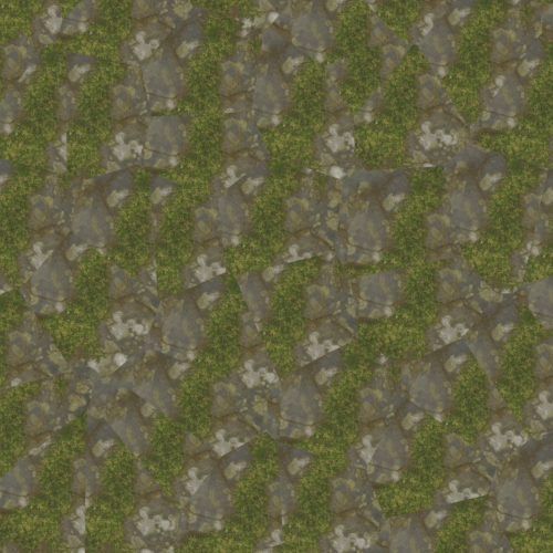
Seamless textures
Using Texture Coordinate and mapping nodes allows us to repeat a given texture a couple of times to reuse it in different places without stretching it too much. It may lead to a problematic repeating pattern of the texture:
One way to solve this problem would be to use a procedurally-generated material instead of a fixed-size texture. Lacking this (and most of the materials you can download online are based on textures), the next best try is to make sure that the repeating parts of the texture are difficult to notice. We call a texture where one cannot distinguish the repeats “seamless”.
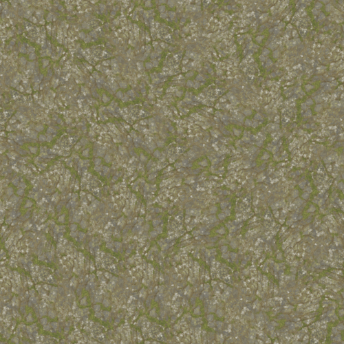
One popular way to achieve this is to use the Voronoy texture, which is a procedurally-generated texture with a number of polygonal cells with different colors.
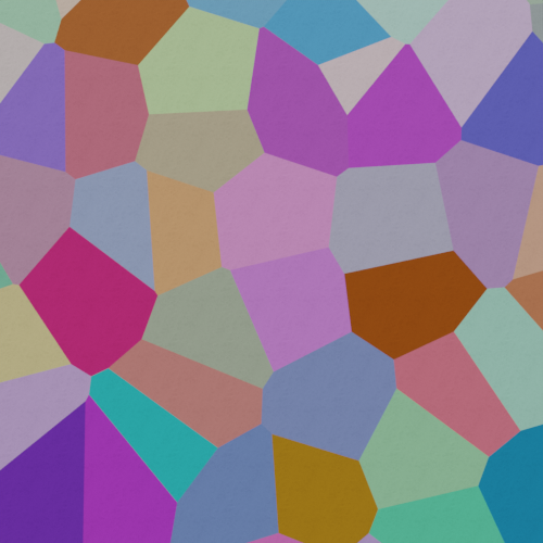
For each pixel in the texture, we are given the (random) color of the current cell and the position of the center of the cell.
To use it for making seamless textures, one needs to put the texture independently in each cell, and apply a random rotation and translation to each of the cells, so that the seams between cells are harder to notice than in a regular grid pattern.
We can achieve it by mapping the UV coordinates to the difference between the UV coordinates and the center of the given cell. This way, the (0, 0) pixel of the texture lies at the center of each cell, and the rest of the cells contain the texture around it7, unscaled.
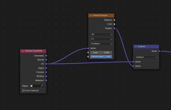
To apply random translation and rotation to each of the cells independently, we can use the random color of the cell, linearly mapped to an appropriate range.
Furthermore, we can add some random noise to the location input of the voronoy texture, making the edges of the cells move around randomly, blurring the edges between the neighboring cells.
More ideas about making seamless textures can be found in this youtube tutorial.
Different textures: vertex groups
So far we discussed applying a single texture to a given mesh. When making a landscape, we often want to use multiple textures, though: there may be a part of the mountain with the forest ground, a part with the rocks, a part with a snowy peak, and so on.
The mechanism that allows us to do this in Blender is called vertex groups. These are 0-1 (continuous!) weights that are assigned to the vertices of a given mesh. This way, we can define which part of the mesh is, say, the forest, and apply the forest texture only there.
As the weights are continuous, we can nicely blend multiple textures. However, it’s generally not possible to mix full materials in Blender, one has to define a single material that combines different shaders based on the vertex group.
Unfortunately, the vertex groups are not directly usable in the shader editor. Instead, one has to make a simple pass-through transformation of the vertex group using geometry nodes, to save the vertex group as a generic attribute which the shader editor can access8. The attribute has to have a different name from the vertex group.
Creating vertex groups
Most of the time, I was drawing the vertex groups manually, roughly marking where different types of terrain would be: as the transitions were mostly smooth, and there are often other elements placed on top of the terrain, the exact placement of the vertex groups doesn’t matter.
One exception to this was the water texture: it would make sense to place the water more in the terrain depressions, but drawing that manually would take a lot of effort.
To avoid that, I used the A.N.T. generator again. Apart from generating the mesh, it also has a “Landscape eroder” functionality, where you can choose some parameters of erosion to apply to your terrain mesh.
The erosion itself wasn’t useful for me, but while generating it the add-on simulates the flow of rainwater in the ecosystem. While doing this, it creates several vertex groups describing where the rain would fall, how the water would flow, and so on. I added the smallest erosion possible to not affect the mesh too much, which generated the vertex groups for the textures as the side-effect.
Particle systems
When creating the landscape mesh, I wasn’t moving each vertex/edge separately, but rather edited it on a higher level of abstraction, changing properties like height, or slope degree in the add-on. Similarly, when I was placing some similar objects in the landscape, like rocks, strands of grass, or trees, I didn’t want to be deciding where to put each of them separately but rather wanted to choose some settings like density, or particular object frequency.
Blender has a modifier, called a Particle system that can be used for randomly placing some objects (particles) on top of a different mesh (emitter).
The particle system modifier is a somewhat old (pre-3.0) way of placing particles. The current Blender version has Geometry nodes9 that allow for expressing emitting particles, as well as many ways for modifying the mesh programmatically, under a common, node-based interface.
However, as geometry nodes are more general than a particle system, setting up a particle system in geometry nodes requires a bit of work, and many settings that are easily accessible from the particle system UI are harder to do in Geometry nodes.
I initially thought that all of the things that I wanted to do related to particles could be expressed using the old-style system, so I decided to use that as opposed to geometry nodes.
Trees
The old modifier worked fine for most of the things: I successfully placed grass, flowers, and rocks. Adding trees ended up being much more time-consuming, though.
I explored some ways of adding individual trees for the particles:
- bringing them as assets from the internet,
- using a popular modular tree add-on,
- making a custom tree generator with geometry nodes.
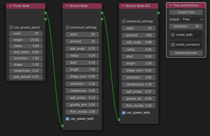
Trees Generator in Geometry Nodes
I started by trying to make a custom tree generator using Geometry nodes. I followed two youtube tutorials (1, 2), which explained the topic well.
While I have learned a lot about how geometry nodes work in the process, the trees that I generated weren’t looking great and were not of the type I was going for.
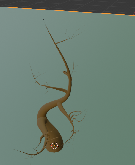
Because of that (and the fact that making the generator was taking a lot of effort), I decided to not progress to adding the leaves but rather explore other ways of adding trees to the scene.
Having said that, after trying other methods I think the idea of using geometry nodes is worth re-exploring, especially by using someone else’s ready-to-use generator from the internet, like this one.
Modular tree add-on
Next, I tried using the modular tree add-on. It’s an old, automatic generator that can make trees of different types. It has a lot of parameters to play with.
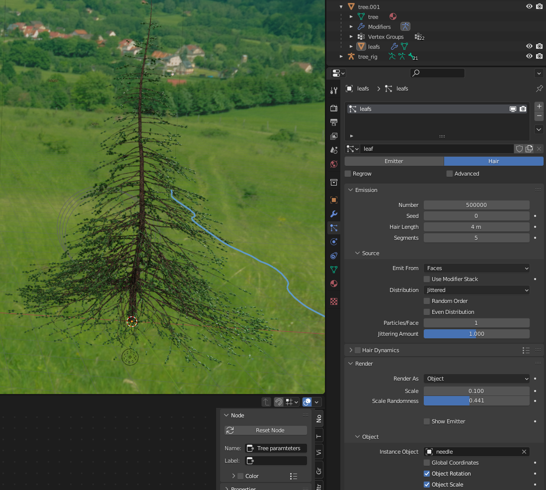
For leaves, the add-on uses the particle system itself: it takes any object as a leaf (actually, twig), and generates settings that use it as a particle to populate around the branches.
Using the trees as particles
Once I had a couple of good-looking trees generated with the modular tree add-on, I tried to use them in a particle system to generate a forest.
This turned out to cause a lot of problems: the particle system modifier doesn’t work well with particles that use a particle system themselves: by default, it will only duplicate the “emitter” (in the case of trees: branches), but not the child particles (leaves).
To fix it, I tried to “apply” the particle system modifier. By default, this only creates the points on which the leaves were meant to be duplicated, but not the leaves themselves.
To get full leaves, one needs to “make particles real” first. This creates a separate copy for each of the particles, which, in the case of leaves, creates thousands of new objects and crashes Blender for me. Ideally, I would be able to ask Blender to make the particles real, but decimate them on the fly, so that I would get a lower-quality version of the mesh without ever creating one with millions of vertices. I didn’t find an option like this.
My next attempt for making the forest was to use geometry nodes, which support up to 8 levels of nested instancing. The problem here was that the nested instancing only works when the outer “instance” (tree) is itself based on the geometry nodes. In the case of the trees generated via the add-on, they were using the old-style particle system, so the nested instancing within geometry nodes didn’t work.
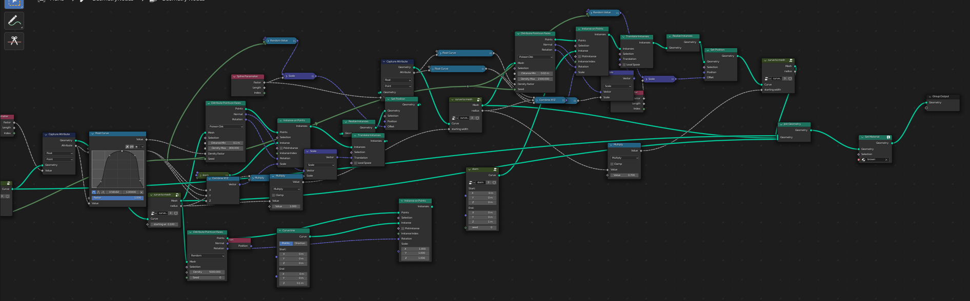
Reproducing particle system in Geometry Nodes
At this point, I decided to try to reimplement the tree particle system in geometry nodes to benefit from nested instances.
Many of the particle system’s settings (e.g. changing density and using a vertex group to mark where to emit the particles) were directly available within one of the geometry nodes.
One problem I observed was that in the particle system when we choose the particles to point towards the normal of the emitter, it will align the local Y axis of the particles with the normal10, whereas for the geometry nodes’ Instance on Points node uses the Z axis.
As the trees were generated for later use in a particle system, one needed to adjust for that. While I could rotate the leaves (and later the trees themselves, as the root was also pointing in the Y, not the Z direction), I tried to force the geometry nodes system to use the same coordinate axes as the particle system one.
After some investigation on the awesome blender stackexchange forum, I learned about the align euler to vector node that allows creating a rotation to point particles to the emitter’s normal along any given axis.
This still wasn’t enough to fully reproduce the particle system’s rotations. While the particles’ Y axes were now pointing along the normal, their rotation along their Y axes wasn’t matching the one in the particle system.
After playing with the two systems a bit more, I realized that the rotation along the normal axis in the particle system is arbitrary (for some of the emitter’s directions) and changes with the rotation of the emitter itself.
It seems like a bug related to the representation of rotations in the particle system: something not worth fixing now that geometry nodes are becoming a new standard11.
Once I was confident that the rotation in geometry nodes was good, I think I would be able to reproduce different features of the particle system modifier there.
However, it turned out that the resulting trees would simply have too many vertices to use as particles: a typical generated tree has around 10 million vertices (even more for a conifer, as you need a lot of needles to cover the tree), whereas to make it work with hundreds of thousands of particles, the most Blender can handle is on the order of 10 thousand vertices per particle.
One needs to find a way to decrease the density of the mesh while ensuring it still looks good. We could achieve it with a Decimate modifier, but it’s not available as a geometry nodes’ node, so we would still have to apply the geometry nodes first, which was too expensive to do before.
Even if the decimation worked, there is a risk that the decimated tree will not look good anymore. So, after spending a lot of effort trying to use generated trees, I decided to use low-poly versions of the trees from the internet, instead of relying on a generator.
Bringing trees as an asset
There are lots of free tree assets available online. They are of varying quality; many of them are generated by the modular add-on itself, so still have the problem with using the particle system and would create too many objects if instantiated.
One can model the tree oneself, but it requires a bit of work (but there are a lot of good tutorials).
What I ended up doing is to try a lot of assets until I found some which are both low-poly and not using the particle systems inside12.
One workflow for creating low poly assets which I didn’t try is to reduce the tree objects from high to low poly (explained e.g. in this tutorial).
Object hiding in a particle system
When using the assets from the internet, I learned about how people implement hiding the base objects in the particle system setup.
When using some object A as a particle in a particle system setting, there are two types of hiding one may want to use:
- to hide the “base” object from rendering in a scene. When we use some object as a particle, its original version doesn’t disappear from the scene; it is still rendered. Unless that’s what we want (and I never wanted that), rendering the base object will waste resources and potentially create some additional reflections of the object.
- To not show the emitted particles in the viewport, to avoid their expensive rendering outside of the final render.
It was easy to find a lot of incorrect advice regarding object hiding (1, 2). What ended up working was:
- to disable the collection with the base object(s). It still appears in the viewport, but not in the renders.
- In the object settings choose:
Object > viewport display > as bounding box.
Wind
Once I added grass, I wanted it to move together with the wind. Blender has a wind force, which is meant to apply some pressure in a particular direction.
When used with the grass and flowers, it didn’t work as well as expected: the movement of the objects was very non-smooth: they would be in a given position for multiple frames, then jump to another position for one frame, then jump back.
It looked like some form of instability in a physics simulation system. I tried to search for it online but wasn’t able to figure out the reason. In the end, I decreased the strength of the wind to very small values which made the effect barely visible.
Wind on the trees
Apart from animating the moving blades of grass, I wanted to animate the tree leaves. For that, I followed this tutorial.
I added a displacement to the leaves’ vertices based on a color in a randomly-generated texture. The position on the texture was controlled by the world-space position of a separate empty object, which can be keyframed as usual.
Lighting
The most physically accurate way for lighting an outdoor scene is to put a single, strong, light source simulating the sun.
Unfortunately, the technical limitations of physics simulation make the light scattering from a single direction not cover the landscape well enough. To make the lighting resemble real scenes more, people use environment maps in a form of High dynamic range images (HDRIs). These are images spanning a half-sphere with an outdoor image, acting both as a background and the source of light.

HDRIs are largely available for free on the same websites that give away the textures with the materials.
Apart from the main light source, artists often add additional, smaller ones, with a varying degree of physical correctness. The main motivation here is to guide the viewer’s eye toward the main character/objects of the scene, separate them from the background, and create the right mood.
I haven’t used the extra lights extensively; I only brought one light to focus the character in the mountain render. Here is a tutorial on lighting that I found useful.
Volumetric effects
The role of the light sources is to generate new light rays that scatter from different objects.
Depending on the type of the atmosphere (i.e. a clear-sky mid-day, or a foggy morning), these light rays will move differently. Furthermore, the way that light travels in an atmosphere with a lot of humidity makes further-away objects appear more blue-ish (atmospheric perspective).
We can simulate similar effects in Blender.
To achieve atmospheric perspective, one can use a simple compositor effect by rendering a separate “distance from the camera” layer and adding it, multiplied by the atmosphere color, to the final render. I used it to achieve an impression of dirt hanging in the air in the desert scene.
A more physically accurate way of simulating this effect can be achieved by using a Volume Absorption shader. It takes a form of a material one can apply to a simple box that encompasses the whole scene, which absorbs the light of a given color which leads to the effect of further-away objects having their colors tinted.
Volume Scatter is a related node that scatters the rays, allowing to simulate an effect like fog or god rays.
Clouds
Apart from the clouds being present on an HDRI, one may want to have clouds inside of the scene.
I saw it being done in three different ways:
- By adding an animated image of the cloud as a flat plane. As long as the camera is not moving too much, it looks surprisingly good (on the tutorials on youtube), but I had a problem finding nice, alpha-transparent gifs of the clouds on the internet.
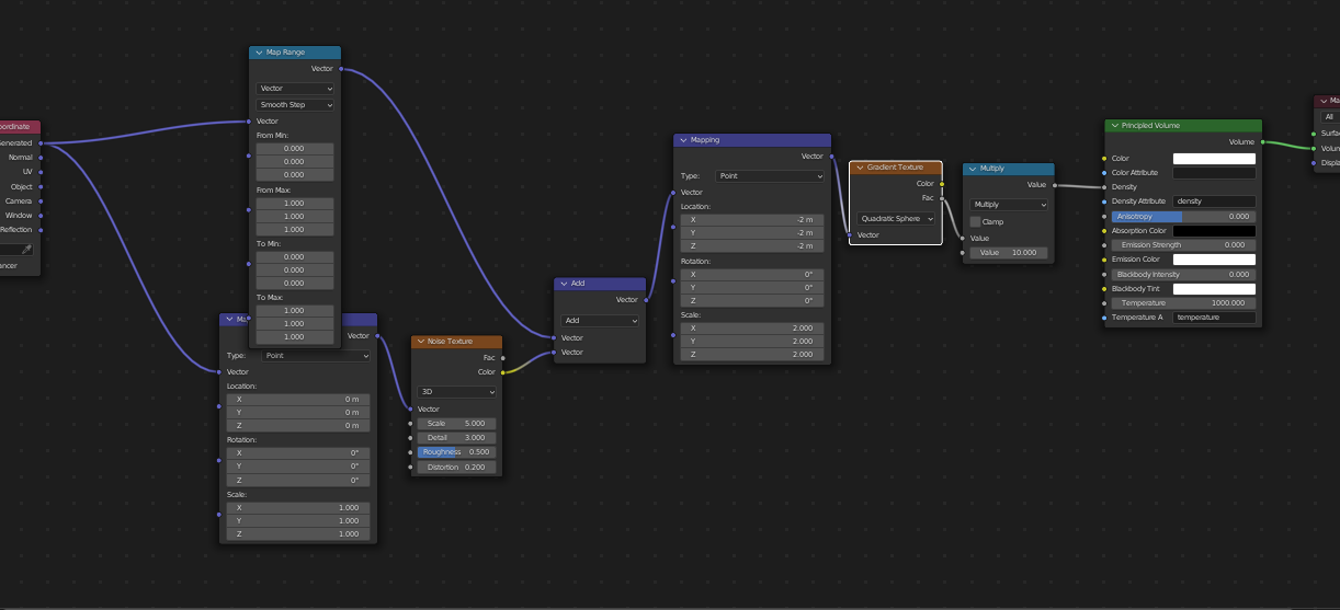
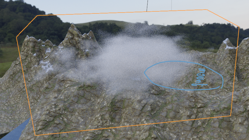
- By procedurally generating a cloud using a Principled Volume node. I used it for one of the clouds in the mountain scene. On its own, the cloud looked good, but I wasn’t able to change the type of the cloud well enough for it to match the background.
- By bringing a random, animated texture on a plane between a light source and the landscape to simulate the shadow of moving clouds. This required adding another light source and balancing the total amount of light, but overall was a relatively simple process with a nice final effect.
Moving the clouds in the sky
Initially, I added the wind to the grass and the tree leaves but kept the HDRI with clouds fixed in place. It created an effect where something feels wrong, but it’s not clear what it is.
When a friend13 pointed the problem out to me, I tried to rotate the HDRI to move the clouds in the sky. Unfortunately, this also moved the background mountains, which looks totally wrong.
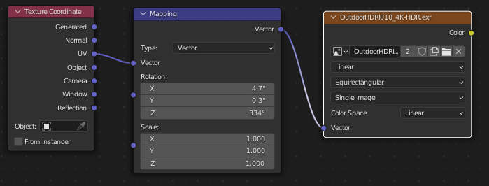
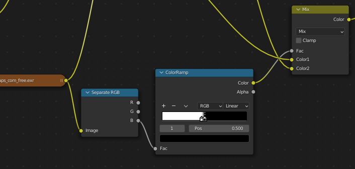
Initially, I thought that I’ll have to edit the HRDI image to split it into the sky and the rest to be able to rotate only a part of it. Luckily, it turns out that the blue channel of the HDRI is significantly stronger for the sky than for the mountains and one can select the sky based on that instead.
In the end, I created two copies of the HDRI texture node and combined them in a Mix Shader using the blue channel as the factor. This way, I could rotate (and animate) only the sky part of the HDRI (which corresponded to one of the texture node copies).
In the image, there was a small bit of an overlap between the “sky” part and the “mountain” part, which caused a thin outline of the mountains to be rotated together with the sky. To avoid this effect, I moved the sky texture a little bit down to hide it behind the mountain part so that the visible part of the sky could be freely moved.
Character
Modeling characters, especially their faces, is very hard: people have thousands of years’ worth of evolutionary experience recognizing other people’s faces and silhouettes, which makes them hard to fake.
Fortunately, there is a website: Mixamo that not only provides reasonable-quality human models for free but also gives many animations for them.
The models are using a common rig system, and the animations are defined using that rig. This way, one can combine any animation with any model and Mixamo will generate the correct animated model. I think it’s even possible to bring one’s own 3d model (assuming that it has the rig attached correctly) to use their animations, but I haven’t tried it yet.
In the two scenes that I made, I took the characters from Mixamo. As the faces of the models were not as good as I would like and the main goal was to show the landscape, I made the characters in the shots face away from the camera.
Camera settings
Camera objects in Blender simulate how a real-life camera/video recorder works. There are several camera settings one can change; two of them that make the most significant effect are focal length and depth of field.
Focal length
Focal length of a lens is a distance from it where the parallel light rays converge, after being refracted by the lens.
The effect on the final image is the amount of perspective distortion: a smaller focal length makes the lines which are parallel in reality converge quicker (i.e. with a smaller angle between them) compared to higher focal lengths that cause the further away objects to seem to have a more identical size.
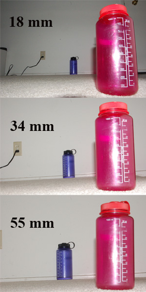
Due to the relative lack of perspective distortion, the images rendered with higher focal lengths tend to appear more flat / less 3D. This effect is more visible when rendering smaller scenes where there would be multiple objects or buildings with parallel lines than in landscapes, though.
The standard focal length used in photography is 35mm. In the two scenes I rendered, I used 35mm focal length for the mountain one and 65mm for the desert one.
Depth of field
The “hole” through which the light travels in a camera is called an aperture. Choosing the size of the aperture is a tradeoff between the amount of light that enters the camera (less light makes it harder to expose the film), and the sharpness of the image (big apertures cause the image to become blurry). You can observe the latter effect in this blog post (at the bottom of the linked section).
With a simulated camera, we don’t have the exposure problems: we can generate as many light rays as we need and make them go through an infinitesimally small aperture. The produced images will look wrong, though, as humans are used to partially-blurry images.
The amount of blurriness is formalized through a notion of depth of field.
In Blender, one can control it through aperture’s F-stop. To choose which object should be in focus, there is a convenient setting that makes a given object (e.g. an empty) define the focal point of the image.
For making animations, one often wants to move the camera to change the focused object or create a particular feeling. There are a lot of good tutorials related to cinematography on this topic (e.g. this one). On the technical level, moving the camera in Blender is easy, as you can keyframe its positions and rotations like for any other object.
Assets
As a final touch, adding high-quality assets close to the camera can help to make the scene more realistic.
One can laboriously model them oneself, but there are lots of websites where the assets are available for free:
- Sketchfab: probably the biggest website with free assets. Some of them are paid, but most of them are available on the CC BY-SA license which requires only to attribute the author in derived work.
- Blend Swap: a website with fewer models but provided as .blend files which can be directly imported to Blender. Non-blender formats like .obj or .fbx sometimes require a bit of work to import them correctly.
- BlenderKit has even fewer models than Blend Swap, but on the other hand provides a very convenient add-on, that allows browsing the assets directly in Blender and importing them via drag-and-drop. It significantly speeds up the asset workflow. Unfortunately, the add-on is not supported very well, and I encountered bugs that crashed it on one of the scenes.
- Megascans. In theory, this is mostly a paid website made by a company called Quixel, which created lots of high-quality models using photogrammetry: automatic generation of 3D models from pictures. Quixel has recently signed a deal with Unreal Engine to allow usage of their models in that engine for free. Theoretically, using the models in Blender wouldn’t follow the license rules, but it’s technically possible. The models come in various “Levels of detail” allowing one to choose higher-density models when placing them close to the camera and lower-density ones when used as particles for further-away areas.
One problem with using the ready assets from the internet is that they limit creative freedom: one won’t be able to do everything they would like because of the lack of the assets.
It’s a skill to know when to let it go and change the vision versus keep searching for the assets that would match the original idea. The reason I didn’t do a wingsuit jump in the mountain landscape, as I initially planned, was that I couldn’t find the right assets.
Other tips
Each of the previous sections has concentrated on a single topic related to building a 3D landscape in Blender. Here, I gathered a few random thoughts that didn’t fit into any particular section.
There are two landscape tutorials, both from CG Boost that I found very useful for a general overview of the whole workflow: Large-Scale Environments in Blender and its newer version: Environments with Geometry Nodes in Blender. Each of them was meant to form a table of contents for a full, hours-long environment tutorial that the author is selling, but they covered everything in enough detail for me, and I don’t think the full course would give me much more.
Apart from these, the same author14 has two more tutorials that I liked: Intro to Compositor, which discusses Blender compositor for combining multiple partial renders and adding post-processing effects, and 6 Tips to Make Your Renders Instantly Cooler.
The tips that the latter tutorial was advertising were to add:
- a blurred foreground element near the borders of the image to add depth to the scene.
- cloud shadows. I explained this in the previous section.
- god rays. I mentioned this in the same section. When I was trying them out, I didn’t manage to make them work well enough when using the shader. Here, the author said to make them as a 2D image, but I didn’t want to be creating new assets for this project.
- falling leaves. I think it would be useful to learn how to use particle systems (or, even better, geometry nodes) to create animated objects, and affect them by the wind, but this didn’t fit my scenes well.
- birds. I saw this advice in multiple places; having flying birds in the scene makes it more lively and adds to the sense of scale.
- atmosphere. I was doing this with volumetric scatter above.
Another tip that I learned when doing these projects was that Blender’s rendering system doesn’t fully ignore data even when it’s unused for rendering. I had Blender crashing or being much slower after adding some heavy objects or materials even when they were turned off. The lesson is to clean up the scene tree from time to time.
Showoff
Here are the two final renders I created:
Desert
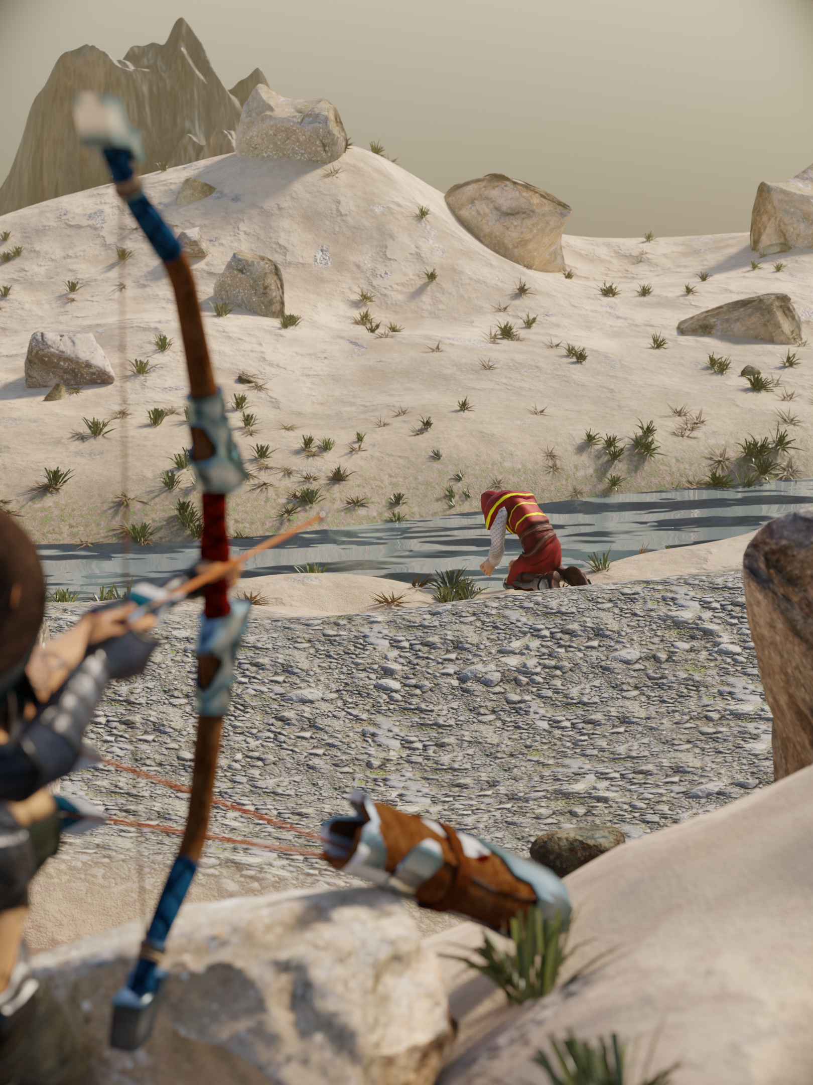
Initially, this was meant to be an animation with an arrow flying, but after doing the single frame the Blender file was messed up so much that I decided to finish it here.
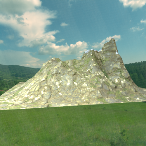
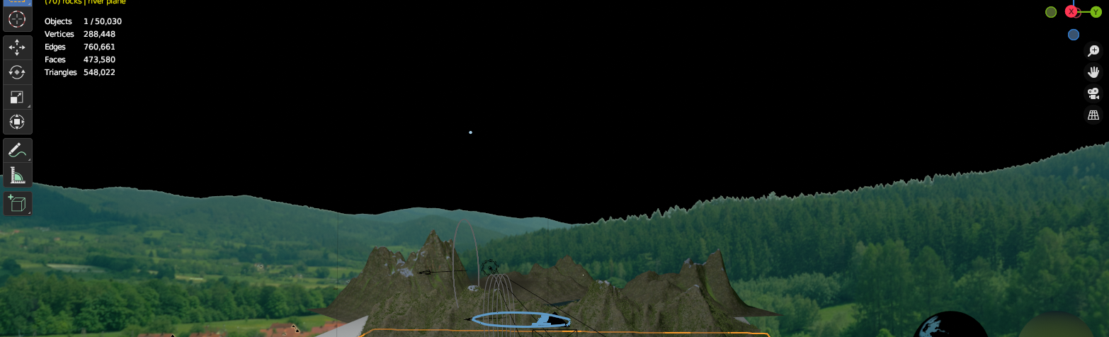
Mountain
Apart from going away from the squirrel guy, originally I was planning that the shot will look at the mountains more from the top. However, when I tried this out, I realized that I would need many smaller mountains to cover the background if I decided on such an angle, so I changed my mind.
The (usually) small box with the parameters of the recently-finished operation, allowing to modify them.↩︎
this youtube tutorial explores wave generation in depth↩︎
see my previous post on how the metallic material property works↩︎
i.e. 4096x4096 or 8192x8192 pixels.↩︎
an alternative would be to create a function that defines color using a mathematical function↩︎
Note that as the coordinates are 3D, the last dimension is ignored if passed to an image texture. One can use these coordinates for other purposes, though.↩︎
the textures are typically wrapped around (0, 0), such that negative “coordinates” correspond to the positions at the other end of a rectangular texture.↩︎
which I discussed in this blog post↩︎
each object in Blender has its own, local coordinate system↩︎
it would still be interesting to understand better the Blender’s rotation coordinates system, but it’s a topic for another post↩︎