Geometry nodes
Blender recently introduced a new way of manipulating 3D meshes: geometry nodes. It combines a standard node-based UI (similar to the one used for constructing materials) with a script-like expressiveness to control each vertex arbitrarily. I learned the basics of geometry nodes and did a simple project using the new mechanism to try them out.
Attributes and domains
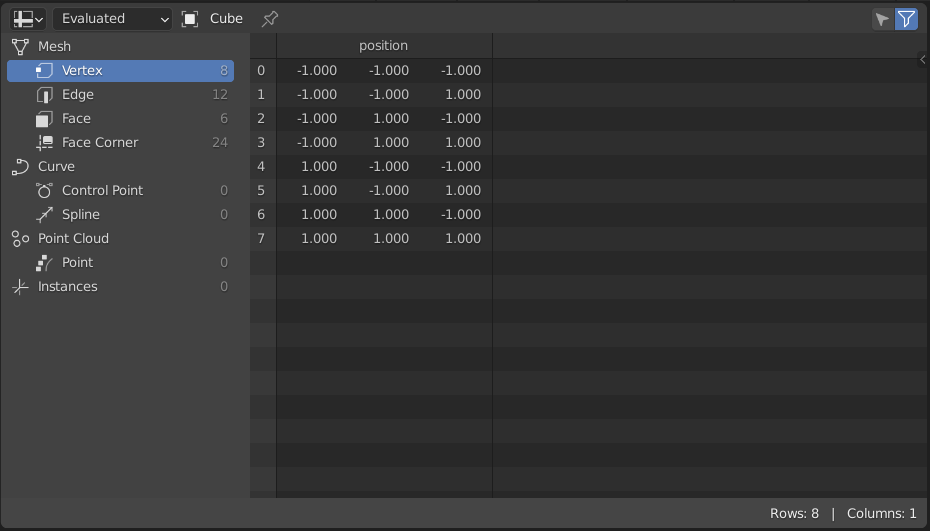
Internally, Blender represents objects using a couple of matrices. There is a description of a single entity (vertex, edge, face) in each row of such a matrix. Each column corresponds to a single attribute: a property of that entity, e.g., its position.
There are as many such matrices as there are types of entities (also known as domains): one for vertices, one for faces, etc.
This representation isn’t very convenient to use, as operating on a set of numbers is usually not as intuitive as making changes in the UI.
With geometry nodes, the changes to the underlying representation can be made more directly than using the standard workflow. Apart from modifying the built-in attributes like position, they allow us to define our own (e.g. color), which are then processed using the same operations as for the built-in ones.
Types of nodes
Geometry nodes is a modifier of an existing object: it processes the elements (vertices, edges, etc.) and the attributes (position and custom attributes) of an object in more or less sophisticated ways using nodes. These elements and attributes together are called a geometry.
There are three types of nodes:
- data flow nodes
- input nodes
- function nodes
Blender uses a joint name of fields for the functional and input nodes.
Data flow nodes
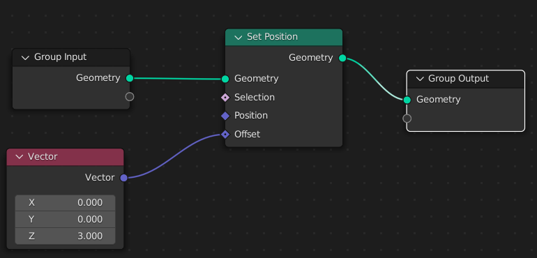
Data flow nodes, which are marked by a green title bar, modify underlying geometry by performing the typical Blender operations like moving, joining two meshes together, or creating new objects.

Input nodes
Input nodes, with red title bars, allow getting some piece of information (stored in the geometry or provided by the user in another way) to be later processed.

Function nodes
Function nodes, having blue title bars, process data that comes in, and return some output.

Eager vs lazy execution
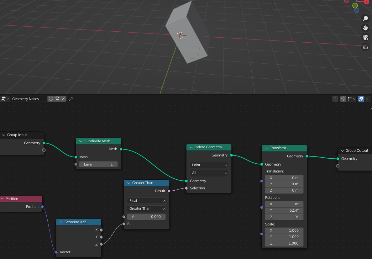
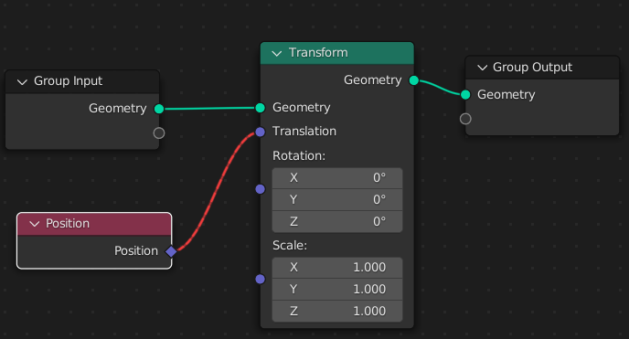
An attentive reader will see that the Position node shown above doesn’t get geometry as an input, even though it reads the positions stored on some geometry.
The incoming geometry is often processed in multiple stages, creating several intermediate geometries before getting the final one. Which one Position node queries for the position of its elements?
To answer this question, one needs to introduce the concept of lazy execution. When we typically think about programming, we are using a mental model of eager execution: there is a number of steps, an algorithm, which we follow from a to z.
In geometry nodes, it would correspond to the nodes being evaluated from left to right: from the ones with no inputs (so we can calculate their outputs) to their children, and so on, until the output node.
For efficiency reasons, geometry nodes don’t work like this. Instead, Blender processing system starts execution from the final output node. It looks for the inputs that need to be calculated to evaluate the node’s output, and so on until it reaches nodes with no inputs. It is called lazy execution.
This way, if some nodes are not necessary to get the output (e.g. because we added them to the system but didn’t use them in the end), they won’t be calculated, saving precious milliseconds at the cost of a less intuitive computation model.
Note that a similar graph-based, lazy execution system was used in TensorFlow 1 to evaluate neural networks.
Coming back to the question of choosing the geometry for the Position node: the geometry used will be the last geometry encountered while lazily-processing the execution; in other words, the one closest to the Position node.
In particular, if we connect a single Position node to multiple geometries, it will provide different outputs for them.
Transferring attributes
Sometimes, we want to combine attributes living on multiple geometries, e.g. when we select a piece of geometry based on some attribute, transform it, and then do another transformation using the original selection (and not based on a new geometry).
There are two ways to use attributes on a different geometry than the one they were originally defined on: transfer and capture attribute.
Transfer attribute
When using transfer attribute, we take one geometry and an attribute that lies on another geometry, and we copy the attribute to the target geometry to use it there.
How to “copy the attribute” when the number of elements in the geometries differs? It is resolved by matching the target geometry with the nearest entities of the source geometry and copying the attribute values from them.
Capture attribute
An alternative, capture attribute, is used when we don’t pass the attribute to another geometry but merely request for the attribute on the current geometry to be preserved for later use.
The capture attribute node takes and returns a geometry to lock the value of an attribute value in place, preventing its re-evaluation on a different geometry further down the chain.
How does the “preservation” work here, when the geometry where we captured the attribute and the one where we use it contain different elements?
Here, as opposed to transfer attribute, we don’t evade doing the transformations to the captured attribute. Whenever the geometry is changed by some functions, the same transformations are applied to the captured attribute as to the other attributes (e.g. position), potentially creating new geometry elements with an appropriate value of the captured attribute.
Capture attribute is particularly useful before transformations that drop some attributes, like Curve to mesh that drops Curve parameter input attribute. With capture attribute, we can lock this attribute to live on the geometry, despite the transformations that are happening to it.
Comparison
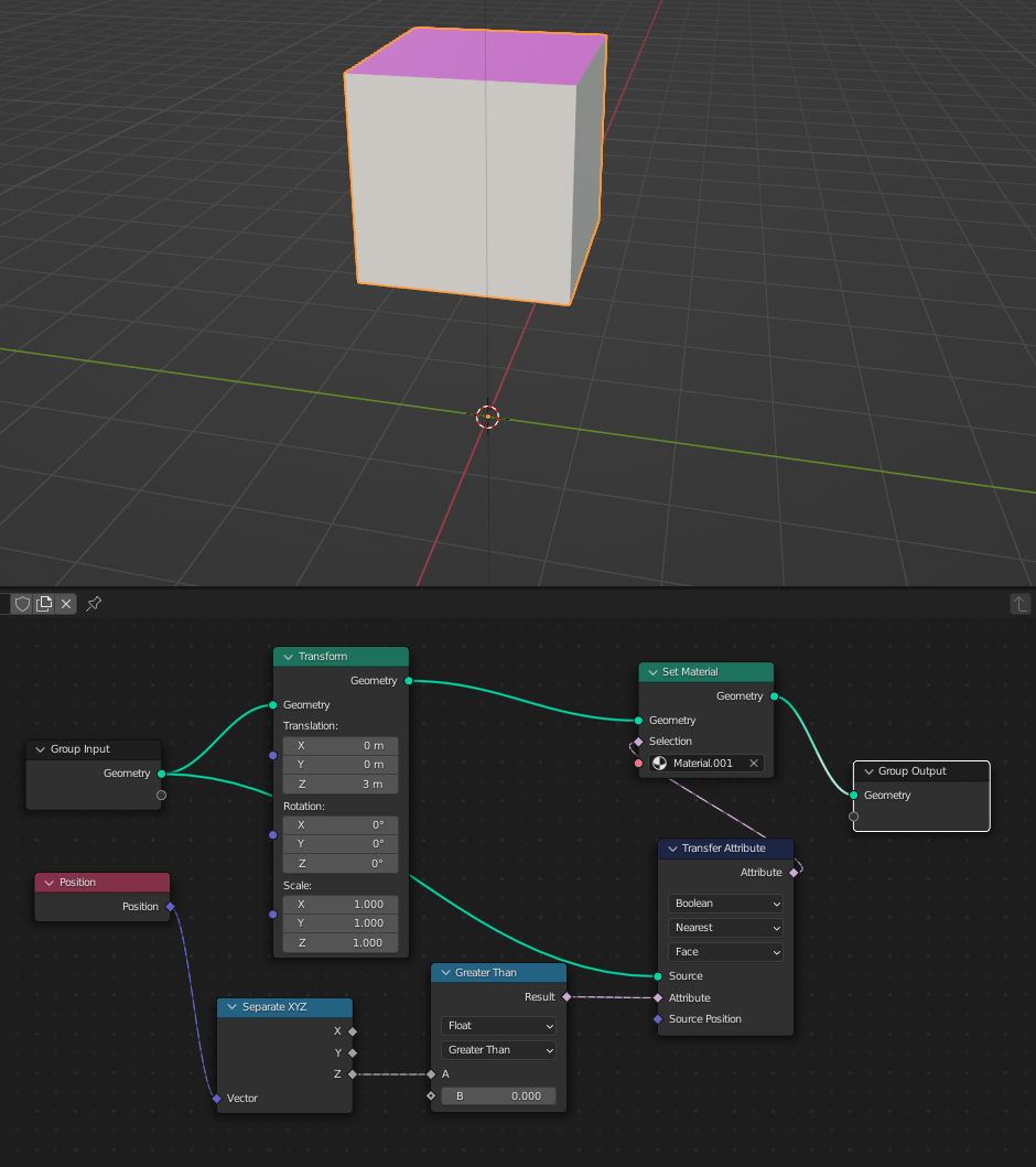
The behavior of transfer and capture attribute can be confusing. To give an example of a situation where their behaviors differ, imagine a scene where we select the top half of a cube, mirror the cube horizontally, then paint the selected part.
With no transfer or capture attributes, the bottom part will be painted: the selection has been reversed and painted afterward.
If we used capture attribute after the selection, the behavior won’t change: the bottom part will be painted. The selection, stored in capture attribute, doesn’t affect the position attribute, which is changed as usual in the mirror reflection.
On the other hand, if transfer attribute is used, the paint will invert. When choosing the selection to paint, Blender will search for the values of the selection in the original geometry, before the mirror reflection. The reflection will cause the vertices to reorder, but their associated values of the selection won’t change, as they are assigned from the nearest vertex in the original geometry. This will make the mirror reflection to not affect the painted part, so only the top will be painted.
Nodes’ sockets
The sockets of the nodes have various colors and shapes.
The color marks the type of the data coming in:purple
for 3D vectors,grey
for scalar floats,pink
for booleans, and others.

The shapes of the sockets correspond to whether the incoming/outgoing data is provided per geometry element (one value per vertex, edge, etc.) or per the whole geometry (e.g. object origin).
The first one (data varying per geometry element) is marked by a diamond, and the socket accepting single data has a shape of a circle.
Instances
Apart from geometry domains of vertices, edges, and faces, geometry nodes handle instances.
They are useful to speed up the processing of multiple identical objects at once: instead of constructing a lot of independent vertices and edges, Blender creates a given instance once and then copies the resulting geometry when needed, similarly to when creating “duplicates” in the UI.
One way to add an instance to the geometry nodes is using an Object info node. It takes an object present in the scene and adds its geometry to geometry nodes.

We can choose whether the geometry should be added “as an instance” or not, in which case the object will be added as separate vertices, edges, etc.
The placement of the new object can be controlled via the Original/Relative setting.
When using Original, the object’s origin (and rotation and scale) is put in the same place as the origin of the object which has the geometry nodes modifier.
When using the Relative setting, the new object is placed such that its location / rotation / scale is the same as it had as a standalone object.
Another node that brings instances into geometry nodes is a Collection info. It works similarly to the Object info one but accepts collections instead of single objects.
It has two settings:
- Separate children, which changes whether to add the whole collection as a single instance or to have one instance per object in the collection, and
- Reset children, which sets to 0 all the local transformations that the objects in the collection have.
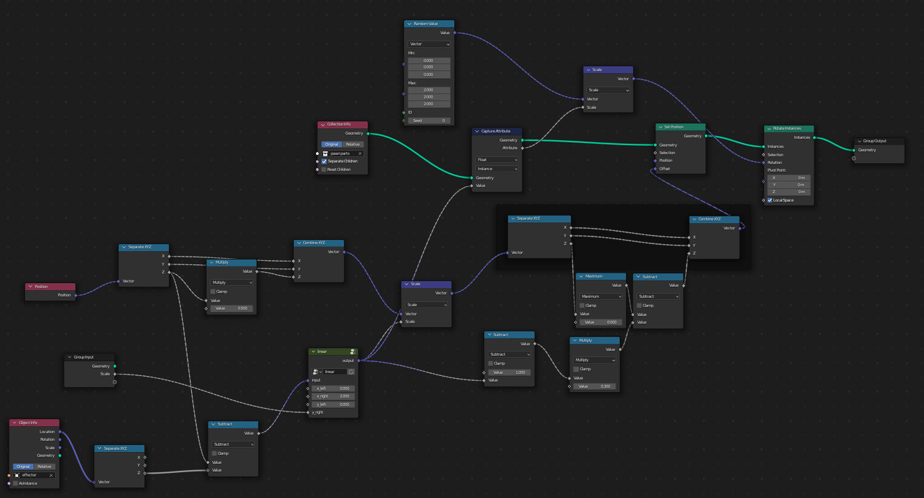
Project: assembling a chess pawn
To experiment with the geometry nodes, I did a small project animating the assembly of a chess pawn from parts.
To divide a pawn (which I modeled in a previous project) into pieces, I used a cell fracture add-on.
Then, I added a geometry nodes modifier to a dummy geometry, loaded pieces from a given collection as instances, and created an empty, which will be driving the animation.
Concretely, the pieces which are significantly above the empty will be spread out and rotated randomly, the ones below will be on their final positions, and the ones close to the Z position of the empty, will be in the process of being assembled.
To create the move, I used a couple of standard nodes, and a capture attribute node to capture the stage of the move of every instance to synchronize the rotation with the move.