Physically-based rendering 101
After watching one of the Two minute papers videos: a short video summary of a research paper made by Károly Zsolnai-Fehér, YouTube algorithm suggested I should watch the rendering course of the same author next. My physically-based rendering knowledge is very fragmented: I was immersed in the lingo without understanding it through friends who are doing PhDs in related areas, and I tried and failed to read PBRT. I watched Károly’s course to connect the dots and, hopefully, to understand Blender better.
Ray tracing
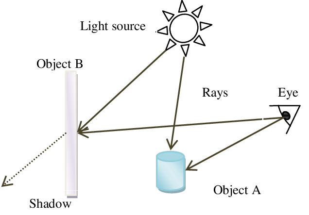
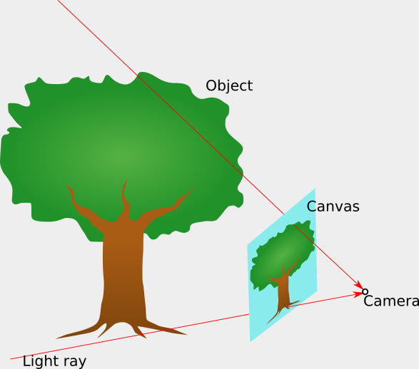
At the heart of physically-based rendering is the ray tracing algorithm. It describes how rays of light travel through a 3D scene:
- light starts at a light source,
- it goes in a straight line to objects, and bounces off them, until
- it hits the camera, in front of which there is a canvas on which the image will appear.
Specular reflection model
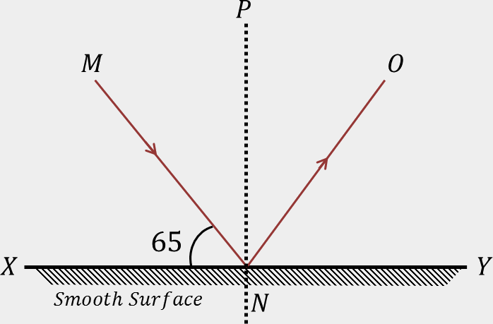
To formalize the above algorithm, one needs to define a model deciding in which direction a light ray reflects from a surface it hits.
One simple reflection model is the specular reflection. It assumes the reflected ray angle to the normal of the surface is the same as the angle between the shining ray and the normal.
If one knows the shapes and locations of objects, lights, and the camera and assumes the reflections follow the specular model, it is easy to calculate the paths of light rays in the scene.
The resulting images would assume that every surface behaves as an ideal mirror, though.
Various materials
The reality is more complex, and there are multitudes of different materials with varying behaviors, like:
- reflecting the light of different colors that makes us see colorful images,
- reflecting rays not in a single direction, but in a range of directions (diffuse reflection),
- allowing (a part of) light to pass through the material after being refracted at the boundary of mediums (e.g. in glass).
BxDF formalism
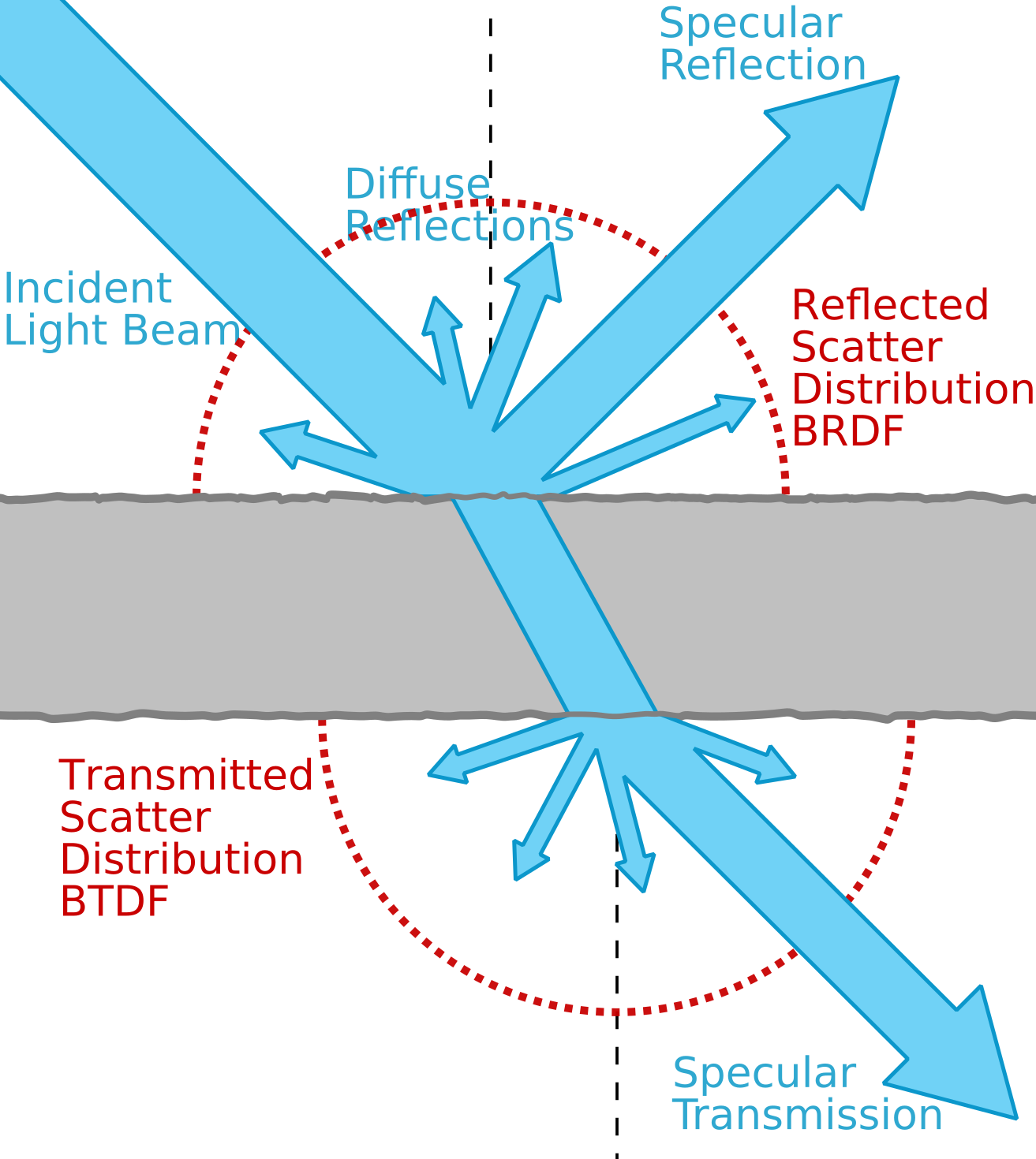
To formally describe the distribution of the reflected light, scientists use a function called Bidirectional Reflectance Distribution Function (BRDF). It is a non-negative function of three parameters
\[f_r(p, \omega_i, \omega_o): R^3 \times [-\pi, \pi]^2 \times [-\pi, \pi]^2 \rightarrow R_+ \cup \{0\}\]
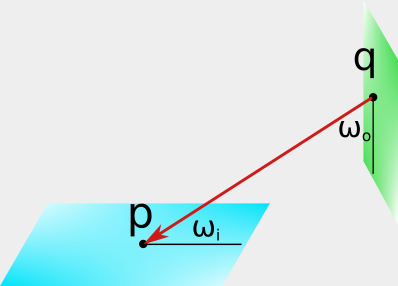
where \(p\) is the point on the surface hit by the ray, \(\omega_i\) is the angle (on the hemisphere) between the incoming ray and the plane tangent to the object in \(p\), and \(\omega_o\) is the angle on the same hemisphere between the outgoing ray and the tangent.
When the value of BRDF is high, a lot of the energy of the ray coming from the direction \(\omega_i\) passes to the ray outgoing in the direction \(\omega_o\); if it is 0, that ray is not reflecting in this direction at all.
BRDF is normalized to behave like a probability density function:
\[\forall_p \int f_r(p, \omega_i, \omega_o) \text{d}\omega_i \text{d}\omega_o \le 1\]
where the integral can be less than 1 to account for the energy loss.
Apart from the light reflected from the surface of an object, we would like to model light passing (transmitted) through partially transparent materials. To do so, we use an analogical function called Bidirectional Transmittance Distribution Function (BTDF) \(f_t(p, \omega_i, \omega_o)\) which describes the amount of energy preserved when light ray coming from direction \(\omega_i\) hits point \(p\) and gets refracted to a direction \(\omega_o\) on the hemisphere on the other side of the surface.
The sum of these functions, describing the two effects together, is called a Bidirectional Scattering Distribution Function (BSDF, \(f\)):
\[f(p, \omega_i, \omega_o) = f_r(p, \omega_i, \omega_o) + f_t(p, \omega_i, \omega_o)\]
Color
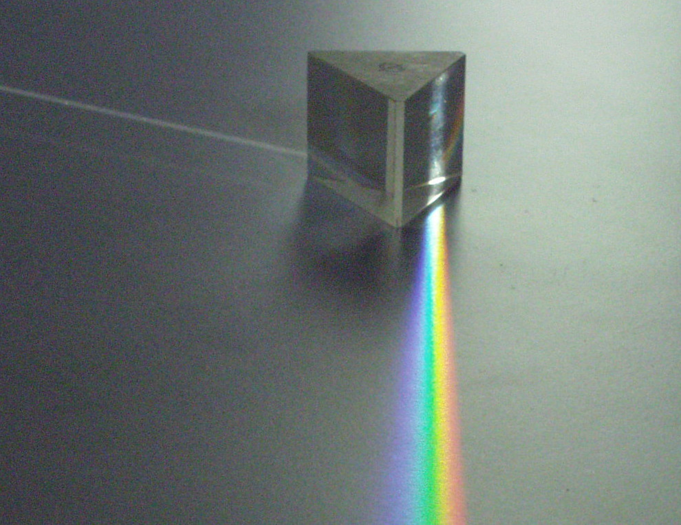
Note that I never mentioned the color in the definitions above. Under this model, we assume that the BSDF (distribution of directions of the outgoing light) is independent of the color (wavelength) of the ray. It is a simplifying assumption that makes it impossible to model situations like dispersion in a prism (where different colors are refracted by a different angle, i.e. need different BSDFs). Nevertheless, it doesn’t affect most of the scenes, and is used in Blender, so we’ll stick with it.
It doesn’t mean that the objects themselves don’t have color, but as handling it is independent from how the light ray travels through the scene, it will be skipped here1.
Rendering equation
How do we use the information about how the light is scattered on various surfaces to draw pixels on the screen?
Under a standard camera model2, the camera is a point, in front of which there is a canvas where the image will appear. The energy of a light ray determines the intensity of the pixel on the canvas that the light ray passed through before reaching the camera.
To model the light shining from a particular point in space, apart from knowing how a single ray scatters locally (BSDFs), we need a way to sum up all the incoming light rays into a single outgoing one. To do this, we use a rendering equation:
\[L_o(p, \omega_o) = L_e(p, \omega_o) + \int f(p, \omega_i, \omega_o) L_i(p, \omega_i) \text{cos}(\sphericalangle(\omega_i, \omega_o)) \text{d} \omega_i\]
Where \(L_o\) is the light outgoing from \(p\) in the direction of \(\omega_o\), \(L_e\) is the amount of the light emitted in that direction (i.e. when \(p\) is a light source), and \(L_i\) is the total light intensity incoming from direction \(\omega_i\).
Note that we can calculate \(L_i\) recursively: to get the amount of light incoming to \(p\) from direction \(\omega_i\), we can find \(q\): the point on the intersection of the incoming ray and the surface nearest to \(p\), and the light incoming to \(p\) from \(q\) will be the same as the light outgoing from \(q\) in the direction of \(p\): \[L_i(p, \omega_i) = L_i(p, \overrightarrow{qp}) = L_o(q, \overrightarrow{pq})\]
If we knew how to calculate the integral in the rendering equation, we could get the angle between a ground plane and the camera - pixel vector for each pixel on the canvas and calculate the light incoming to the camera from that direction: \[L_i(\text{camera}, \overrightarrow{(\text{pixel}, \text{canvas})})\]
using the rendering equation, which would define the intensity of the pixel.
Approximating the integral
As anyone who ever calculated an integral knows, analytically working out an integral is difficult in all but the simplest of cases. Even if we restricted our BSDFs to very simple functions (limiting the properties of materials that we could express), we’d still need to do the calculation recursively over all (generally infinitely many) of the points the light ray can reach.
As the exact solution to the rendering equation is infeasible, we will be looking for an approximate one. The most popular method to do so is Monte Carlo integration.
It is based on the interpretation of the integral as a mean value of the function of a random variable: \[\int_X f(x) \text{d}x = \mathbb{E}_{x \sim X} f(x)\]
Now, instead of calculating the function for every possible value of the random variable \(X\), we can sample it a couple of times according to its distribution and average the value of the function in these points: \[\mathbb{E}_X f(x) \approx µ_N = \frac{1}{N}\sum_{i=1}^N f(x_i), x_i \sim X\]
Of course, the more samples we take (the bigger N is), the closer (on average3) the resulting mean \(µ_N\) will be to the real mean \(\mathbb{E}_{x \sim X} f(x)\). At the same time, the \(µ_N\) estimator is unbiased, i.e. has no consistent skew to be bigger or lower than the true mean.
This leads to an algorithm we can implement. For a given pixel \(p\):
- We find the first intersection point \(q\) on the vector \(\overrightarrow{cp}\) starting in the camera \(c\) and passing through the pixel.
- We sample the new incoming direction (corresponding to \(\omega_i\) in the rendering equation) uniformly from the hemisphere centered in \(q\).
- We recursively calculate \(L_i(q, \omega_i)\), stopping the recursion after a fixed number of bounces (the process would never end otherwise).
- We set the pixel to \(L_e(q, \overrightarrow{pc})\) (positive if \(q\) is a light source) + \(f(q, \omega_i, \overrightarrow{pc})\) (BSDF) times the value of recursively calculated incoming light (\(L_i(q, \omega_i)\)) times the cosine of the angle between \(\omega_i\) and \(\overrightarrow{pc}\).
- As we repeat this process with sampling multiple directions \(\omega_i\) and average the results, the pixel intensity approaches the correct value based on the rendering equation.
Disclaimer on practice
This process, while unbiased (except for the fact that we cut the recursion after a couple of bounces), can require a lot of samples to converge. In particular, for a punctual light, it is effectively impossible to hit it (we would reach it with probability 0).
There are some simple ways to make it more efficient, e.g. by shooting rays from both the camera and the light source at the same time or changing the distribution of rays to a different one than uniform over angles and correcting the resulting integral (importance sampling).
Many PhDs have been written on how to speed up the rendering process. To keep things simple, I’ll assume the model described above, with rays shooting from the camera to approximate the integrals with vanilla Monte-Carlo, even if this is not how one implements a modern renderer in practice.
Artist to math translation
BSDF is a representation of the material that’s convenient for a computer, as it can easily sample outgoing ray directions and quantify the amount of lost energy from the bounce.
Expressing the material in terms of a BSDF is tricky for artists who create 3D models, though: it’s more natural for humans to think about the physical properties like color or glossiness than about the 7-dimensional BSDF.
To facilitate the process of constructing materials, 3D rendering software has nodes that can map physical parameters like “Transmission” or “Roughness” into a BSDF which will be later used by the renderer.
The most popular node in Blender that outputs a BSDF is called Principled BSDF. It is based on a seminal paper from Disney, where they were investigating ways to express a BSDF using a small number of properties understandable by artists.
In the next blog post, I analyze its parameters to see how they influence the produced material.
I plan to do another blog post dealing specifically with various properties of materials, including color.↩︎
Ignoring camera lenses and inversion of the image caused by the pinhole.↩︎
See law of large numbers for a formalization and proof of this statement.↩︎